9 Optimization in R
Actuaries often write functions (e.g. a likelihood) that have to be optimized. Here you’ll get to know some R functionalities to do optimization.
9.1 Find the root of a function
Consider the function \(f: x \mapsto x^2-3^{-x}\). What is the root of this function over the interval \([0,1]\)?
$root
[1] 0.68602

$f.root
[1] -8.0827e-06

$iter
[1] 4

$init.it
[1] NA

$estim.prec
[1] 6.1035e-05
? uniroot
# in more lines of code
f <- function(x){
x^2-3^(-x)
}
# calculate root
opt <- uniroot(f, lower=0, upper=1)
# check arguments
names(opt)[1] "root" "f.root" "iter" "init.it" "estim.prec"[1] -8.0827e-06# visualize the function
range <- seq(-2, 2, by=0.2)
plot(range, f(range), type="l")
points(opt$root, f(opt$root), pch=20)
segments(opt$root, -7, opt$root, 0, lty=2)
segments(-3, 0, opt$root, 0, lty=2)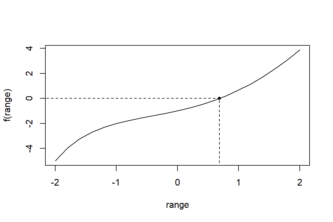
9.2 Find the maximum of a function
You look for the maximum of the beta density with a given set of parameters.
# visualize the density
shape1 <- 3
shape2 <- 2
x <- seq(from=0, to=1, by=0.01)
curve(dbeta(x,shape1,shape2), xlim=range(x))

opt_beta <- optimize(dbeta, interval = c(0, 1), maximum = TRUE, shape1, shape2)
points(opt_beta$maximum, opt_beta$objective, pch=20, cex=1.5)
segments(opt_beta$maximum, 0, opt_beta$maximum, opt_beta$objective, lty=2)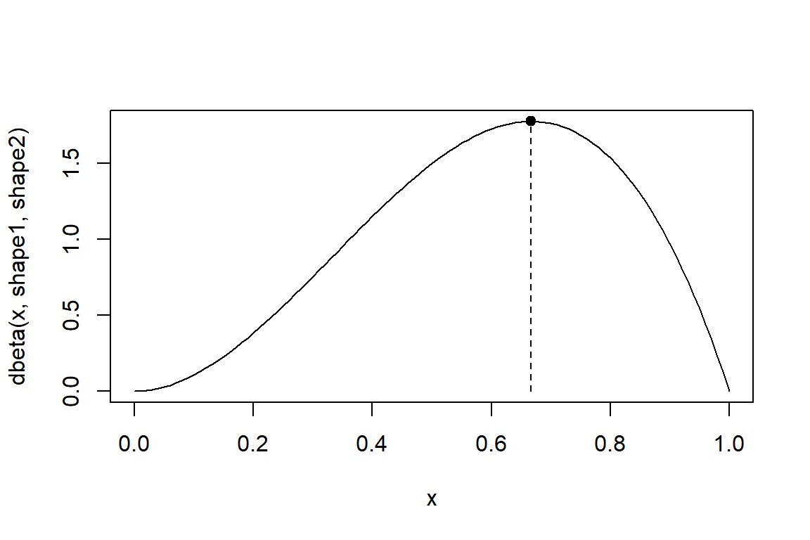
9.3 Perform Maximum Likelihood Estimation (MLE)
Once we know the expression for a probability distribution, we can estimate its parameters by maximizing the (log-)likelihood. Take logistic regression, for example. Here, the likelihood function is given by \[L(\boldsymbol{\beta}) = \prod_{i=1}^{\text{n}} p_i^{y_i} (1 - p_i)^{(1 - y_i)}\] where \[p_i = \frac{e^{\boldsymbol{x}_i^{'} \boldsymbol{\beta}}}{1 + e^{\boldsymbol{x}_i^{'} \boldsymbol{\beta}}}\] and where \(\boldsymbol{x}_i\) is the covariate vector for observation \(i\) and \(\boldsymbol{\beta}\) the parameter vector. The log-likelihood is given by \[\ell(\boldsymbol{\beta}) = \sum_{i=1}^{\text{n}} y_i \log(p_i) + (1 - y_i) \log(1 - p_i).\]
Hence, with a dataset, we optimize this function to get the maximum likelihood estimate \(\hat{\boldsymbol{\beta}}\). To do this in R, let’s use the birthwt dataset from the package MASS.
   low age lwt race smoke ptl ht ui ftv  bwt
85   0  19 182    2     0   0  0  1   0 2523
86   0  33 155    3     0   0  0  0   3 2551
87   0  20 105    1     1   0  0  0   1 2557
88   0  21 108    1     1   0  0  1   2 2594
89   0  18 107    1     1   0  0  1   0 2600
91   0  21 124    3     0   0  0  0   0 2622
We want to model the probability on low birthweight as a function of the variables age, lwt, race and smoke and create an object Form containing this formula to make life easy.
When fitting a logistic regression model, we get the following results.
Call:  glm(formula = Form, family = binomial, data = Df)

Coefficients:
(Intercept)          age          lwt         race        smoke
   -0.21886     -0.02933     -0.00996      0.48349      1.06028

Degrees of Freedom: 188 Total (i.e. Null);  184 Residual
Null Deviance:      235
Residual Deviance: 217  AIC: 227
We will use this to check if we did everything correctly when using our self-written code. We first start by writing a function for the (negative) log-likelihood.
logLikLR <- function(B, X, y) {
  Eta  <- X %*% B
  pHat <- binomial()$linkinv(X %*% B)
  -sum(y * log(pHat) + (1 - y) * log(1 - pHat))
}
Note that we use the negative log-likelihood here. We do this because the functions that we will use minimize our function instead of maximizing it.
When programming, it’s always good to perform some sanity checks. A double or tripple check will assure you that you did not do anything stupid (such as having written a + instead of a -).

Retrieved from https://lefunny.net/funny-sanity-saying/
'log Lik.' -108.54 (df=5)[1] -108.54OK, so that checks out. Noice, let’s go the next step. Now we need a function that minimizes our (multivariate) function for us. For this, we can use the function optim. When using optim, we also need some initial values for our parameters. The log-likelihood for our logistic regression model isn’t overly complex and hence, we can just use 0’s as starting values.
Bstart  <- rep(0, length(coef(glmFit)))
X       <- model.matrix(Form, data = Df)
y       <- Df$low
LRoptim <- optim(Bstart, logLikLR, X = X, y = y)
cbind(LRoptim$par, glmFit$coefficients)
[,1] [,2]
(Intercept) -0.216013 -0.2188631
age -0.028919 -0.0293297
lwt -0.010107 -0.0099619
race 0.486534 0.4834924
smoke 1.057790 1.0602764OK, not bad, but I think we can do better. So let’s use some other optimizers.
LRoptim <- optim(Bstart, logLikLR, X = X, y = y, method = "BFGS")
cbind(LRoptim$par, glmFit$coefficients)
[,1] [,2]
(Intercept) -0.187902 -0.2188631
age -0.029567 -0.0293297
lwt -0.010137 -0.0099619
race 0.481723 0.4834924
smoke 1.060900 1.0602764Euhm, yes, looking good for all estimated coefficients except the intercept. What do we do now? One way to further improve it, is by adding a function that returns the gradient vector. So, let’s do this. Remember that we are working with the negative log-likelihood and that we therefore also have to adjust our function to compute the gradient!
Gradient <- function(B, X, y) {
  pHat <- binomial()$linkinv(X %*% B)
  -crossprod(X, y - pHat)
}
LRoptim <- optim(Bstart, logLikLR, X = X, y = y, method = "BFGS", gr = Gradient)
cbind(LRoptim$par, glmFit$coefficients)
[,1] [,2]
(Intercept) -0.2186091 -0.2188631
age -0.0293351 -0.0293297
lwt -0.0099625 -0.0099619
race 0.4834678 0.4834924
smoke 1.0602591 1.0602764Phew, that looks a lot better! As an alternative to optim, we can use nlm.
[,1] [,2]
(Intercept) -0.2186088 -0.2188631
age -0.0293284 -0.0293297
lwt -0.0099641 -0.0099619
race 0.4834839 0.4834924
smoke 1.0602703 1.0602764We see that the results of nlm are even more accurate without having to adjust the default settings. As with optim, we can also add a function to compute the gradient, but here we have to add it as an attribute in the original function.
logLikLR <- function(B, X, y) {
Eta <- X %*% B
pHat <- binomial()$linkinv(X %*% B)
LL <- -sum(y * log(pHat) + (1 - y) * log(1 - pHat))
attr(LL, "gradient") <- -crossprod(X, y - pHat)
LL
}
LRnlm <- nlm(logLikLR, Bstart, X = X, y = y)
cbind(LRnlm$estimate, glmFit$coefficients)
[,1] [,2]
(Intercept) -0.2188630 -0.2188631
age -0.0293297 -0.0293297
lwt -0.0099619 -0.0099619
race 0.4834924 0.4834924
smoke 1.0602765 1.0602764We can even add the Hessian matrix (and again, remember that we are working with the negative log-likelihood)!
logLikLR <- function(B, X, y) {
  Eta  <- X %*% B
  pHat <- as.vector(binomial()$linkinv(X %*% B))
  W    <- diag(pHat * (1 - pHat), ncol = length(pHat))
  LL   <- -sum(y * log(pHat) + (1 - y) * log(1 - pHat))
  attr(LL, "gradient") <- -crossprod(X, y - pHat)
  attr(LL, "hessian") <- t(X) %*% W %*% X
  LL
}
LRnlm <- nlm(logLikLR, Bstart, X = X, y = y, gradtol = 1e-8)
cbind(LRnlm$estimate, glmFit$coefficients)
[,1] [,2]
(Intercept) -0.2188631 -0.2188631
age -0.0293297 -0.0293297
lwt -0.0099619 -0.0099619
race 0.4834924 0.4834924
smoke 1.0602764 1.0602764