2 Data exploration

In this tutorial you import a dataset and perform an exploratory analysis of the variables. You will visualize the data with ggplot and calculate basic statistics such as the expected value and variance of each variable.

2.1 Importing data in R

The data for this tutorial is stored in the file CPS1985.txt, which is stored in a local subdirectory data. Check out chapter 4 of Data science in insurance: an R intro for a detailed overview of the R methods for importing data.

2.1.1 Determining the file path

Before we can import the data, we have to identify the file location. The file location can be specified by an absolute path or a relative path.

absolute_path <- "C:\\Users\\u0095171\\Dropbox\\Verzekeringen niet-leven\\Bookdown\\data\\CPS1985.txt"
relative_path <- "data\\CPS1985.txt"

Directories in the file path can be separated by a forward slash (/) or a double backward slash (\\).

Relative paths in R always start from your working directory. The command getwd() returns your current working directory.

getwd()

[1] "C:/Users/u0095171/Dropbox/Research AFI/R software/Bookdown/LossModels"

setwd() specifies the working directory for the current R session. Once set, all files in the working directory can be referenced by relative paths.

# This is the map containing all files for the tutorial
setwd("C:\\Users\\u0095171\\Dropbox\\Verzekeringen niet-leven\\Bookdown\\")

# This is a relative path from the working directory to the file we want to import
path <- "data\\CPS1985.txt"

To make sure that the file is located in this directory, we can check it using the command file.exists().

file.exists(path)

[1] TRUE

It is often convenient to set the working directory to the location of the active R file. In Rstudio the following code retrieves the directory of the active document.

dir <- dirname(rstudioapi::getActiveDocumentContext()$path)
setwd(dir)

2.1.2 Organizing your analysis

CheckDir <- function(x) if(!dir.exists(x)) dir.create(x)
pathDir  = path.expand("~/AnalysisLossModels/")
pathData = paste0(pathDir, "Data/")
pathFigs = paste0(pathDir, "Figures/")
pathRes  = paste0(pathDir, "Results/")
sapply(list(pathDir, pathData, pathFigs, pathRes), CheckDir)

[[1]]
NULL

[[2]]
NULL

[[3]]
NULL

[[4]]
NULL

file.copy(path, pathData)

[1] FALSE

setwd(pathDir)
dir()

[1] "Data"    "Figures" "Results"

list.files(recursive = T)

[1] "Data/CPS1985.txt"

2.1.3 Import a .txt file

read.table() is the most basic import function in R. You can specify tons of different arguments in this function (See ?read.table).

We import the dataset CPS1985.txt in a variable CPS.

CPS <- read.table(path)

After importing a dataset, you should always inspect the data to confirm that the data was imported correctly. head prints the first records of the dataset.

head(CPS)

   wage education experience age ethnicity region gender occupation
1  5.10         8         21  35  hispanic  other female     worker
2  6.67        12          1  19      cauc  other   male     worker
3  4.00        12          4  22      cauc  other   male     worker
4  7.50        12         17  35      cauc  other   male     worker
5 13.07        13          9  28      cauc  other   male     worker
6  4.45        10         27  43      cauc  south   male     worker
         sector union married
1 manufacturing    no     yes
2 manufacturing    no      no
3         other    no      no
4         other    no     yes
5         other   yes      no
6         other    no      no

Some more data characteristics:

# nrow returns the number of rows in the dataset
nrow(CPS)

[1] 533

# colnames returns the variable names in the dataset
colnames(CPS)

 [1] "wage"       "education"  "experience" "age"        "ethnicity"
 [6] "region"     "gender"     "occupation" "sector"     "union"
[11] "married"   

2.2 Data exploration

We continue to explore the variables in the CPS dataset with a focus on wage and sector.

2.2.1 variable types

The same data can often be stored in different formats. The function class returns the type of an R object.

Use the function class to

1. Determine the class of the dataset CPS;
2. Determine the class of the variables wage and sector in the dataset CPS.

# @1. 
class(CPS)

[1] "data.frame"

# @2.
class(CPS$wage)

[1] "numeric"

class(CPS$sector)

[1] "character"

Within the tidyverse the class of all variables in a dataset can be determined using map_chr(<dataset>, class).

The function map(<dataset>, <function>) applies <function> to each of the columns of <dataset>. We can use map_chr when the output of <function> is of type character.

require(tidyverse)
map_chr(CPS, class)

       wage   education  experience         age   ethnicity      region
  "numeric"   "integer"   "integer"   "integer" "character" "character"
     gender  occupation      sector       union     married
"character" "character" "character" "character" "character" 

2.2.2 Factor variables

factor is the R-datatype for unordened categorical variables.

Some usefull functions for factorvariables are:

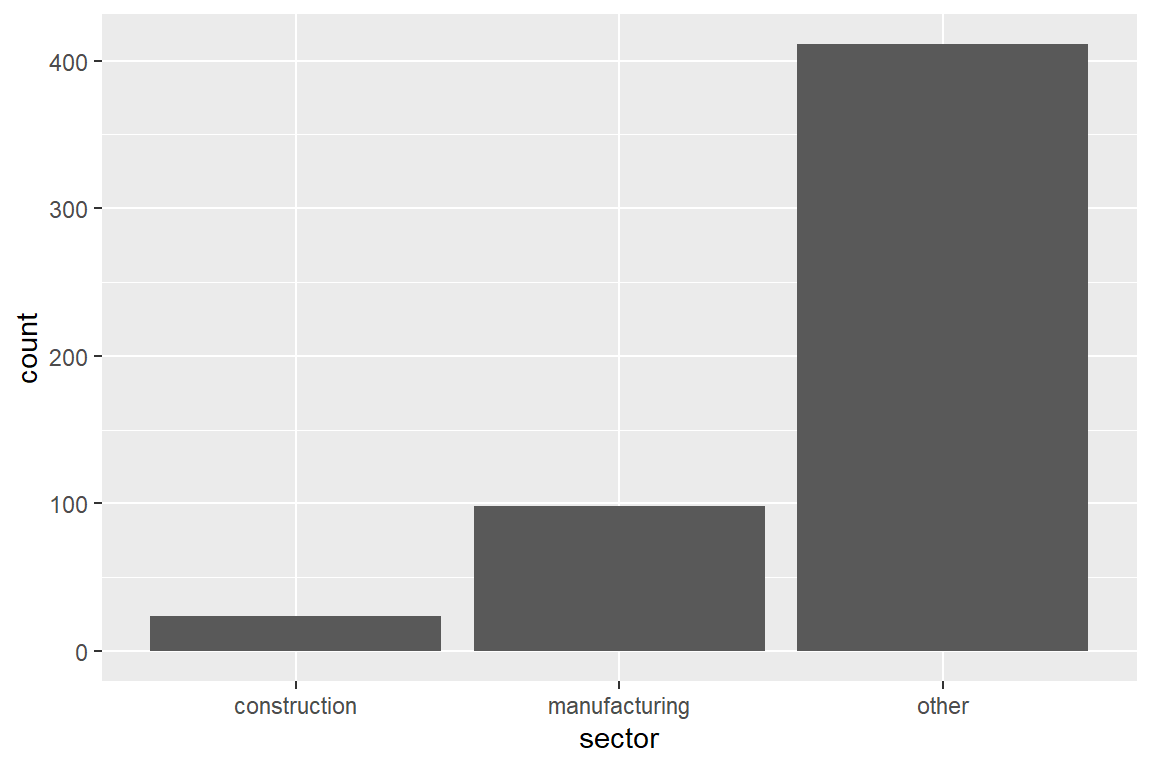
• levels: shows the possible outcomes.
• table: shows the frequency of the possible outcomes.

levels(CPS$sector)

NULL

table(CPS$sector)

 construction manufacturing         other
           24            98           411 

Factors are type-safe, that is you will get a warning when you try to insert a value that is not in levels(<factor variable>).

test <- CPS$sector
test[1] <- 'insurance'

head(test)

[1] "insurance"     "manufacturing" "other"         "other"
[5] "other"         "other"        

table(test)

test
 construction     insurance manufacturing         other
           24             1            97           411 

NA values are an indication that some calculation went wrong. Notice that the NA value is not shown in the output of table. To obtain the number of NA observation use sum(is.na(<dataset>)).

sum(is.na(test))

[1] 0

To insert a new value in a factor variable, we first adapt the set of allowed outcomes.

levels(test) <- c(levels(test), 'insurance')
table(test)

test
 construction     insurance manufacturing         other
           24             1            97           411 

test[1] <- 'insurance'
table(test)

test
 construction     insurance manufacturing         other
           24             1            97           411 

The following code applies table to all columns of the dataset CPS that are of class factor.

require(tidyverse)
CPS %>% 
  keep(is.factor) %>% # Select all columns of class factor
  map(table) # apply the table function to these columns

named list()

In ggplot, geom_bar is used to construct barplots. Check out the online documentation for examples.

require(ggplot2)
ggplot(CPS) +
  geom_bar(aes(sector))

Adding fill = <second factor variable> visualizes the interaction between two factor variables.

ggplot(CPS) +
  geom_bar(aes(sector, fill = gender))

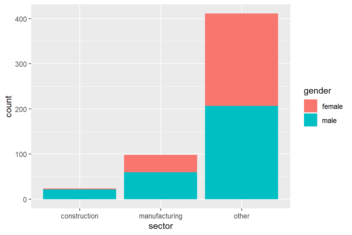
The default behavior is to stack bars. Adding position = position_dodge() shows bars of different color side-by-side.

ggplot(CPS) +
  geom_bar(aes(sector, fill = gender),
           position = position_dodge())

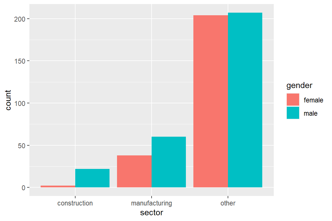
The following code visualizes the distribution of sector by gender.

ggplot(CPS) +
  geom_bar(aes(sector, 
               fill = gender,
               y = ..prop..,
               group = gender),
           position = position_dodge())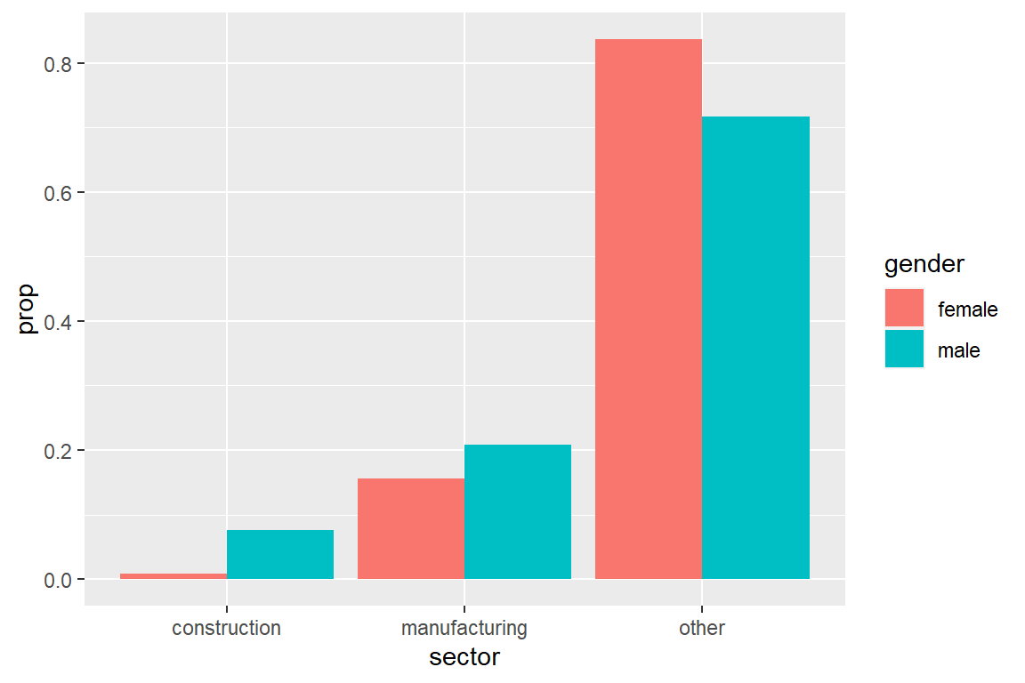

2.2.3 Numeric variables

The variable wage in the dataset CPS is numeric.

class(CPS$wage)

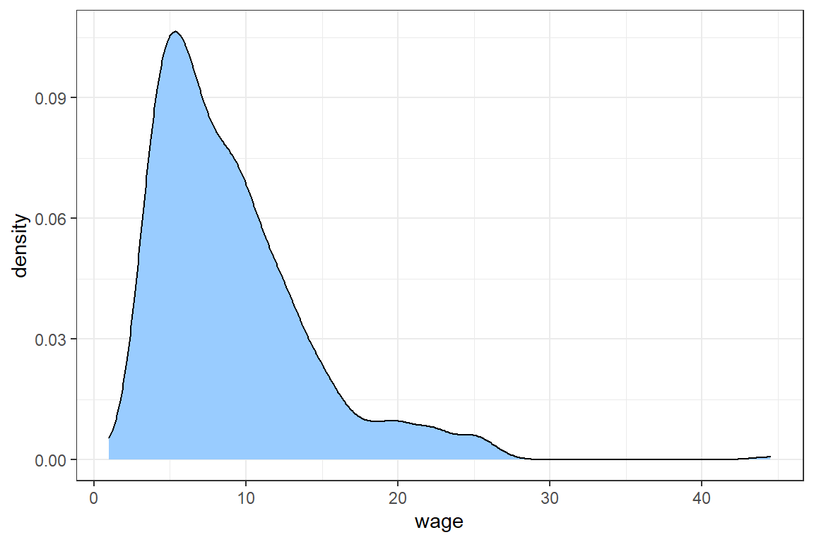
[1] "numeric"

A good strategy is to start by visualizing numeric variables in a density plot.

ggplot(CPS) +
  theme_bw() +
  geom_density(aes(wage), fill = "#99CCFF")

Adding theme_bw() selects the black and white theme for ggplot figures.

The density shows that most wages are between 0 and 30, but there is an outlier with a wage of more than 40.

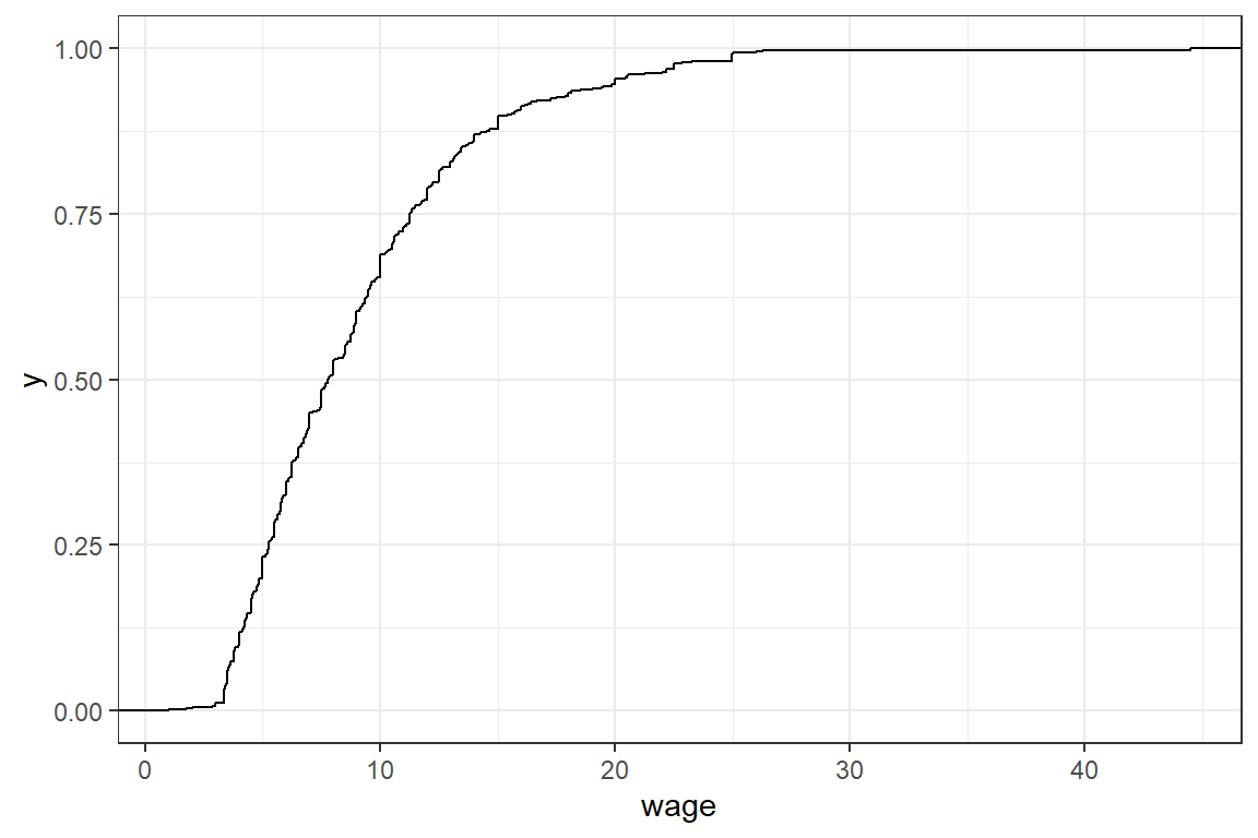
stat_cdf visualizes the empirical cdf.

ggplot(CPS) +
  theme_bw() +
  stat_ecdf(aes(wage))

mean and sd calculate the empirical mean and standard deviation of a numeric variable.

mu <- mean(CPS$wage)
sigma <- sd(CPS$wage)

print(c(mu, sigma))

[1] 9.032 5.141

You can also calulate the mean and standard deviation using the formulas \[\mu = E(X) = \frac{1}{n}\sum_{i=1}^n x\] and \[\sigma = \sqrt{E((X-\mu)^2 } = \sqrt{\frac{1}{n}\sum_{i=1}^n (x-\mu)^2}\]

n <- length(CPS$wage)

# mean
sum(CPS$wage)/n

[1] 9.032

# sd
sqrt(sum((CPS$wage - mu)^2)/n)

[1] 5.136

There is a slight difference between our outcome and the result of sd(.), since the latter divides by n-1 instead of n.

We test whether the normal distribution is a good approximation for CPS$wage. For this we visualize the density of CPS$wage and its normal approximation in a single graph.

In order to visualize the normal approximation we simulate 1000 observations from a normal distribution with the same mean and standard deviation as CPS$wage.

normal_approx <- rnorm(1000, mean = mu, sd = sigma)

rnorm generates observations from a normal distribution.

ggplot() +
  theme_bw() +
  geom_density(aes(CPS$wage, fill = 'original data'), alpha = .5) +
  geom_density(aes(normal_approx, fill = 'normal approximation'), alpha = .5)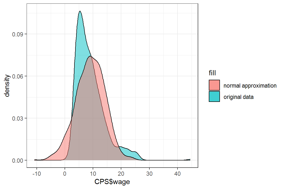

The shape of these densities is quite different and we conclude that the normal distribution is not a good approximation for CPS$wage. One of the reasons for this poor approximation is that the normal distribution is defined on \([-\infty, \infty]\), whereas wage has to be positive.

We transform the outcomes of CPS$wage by taking the logarithm.

log_wage = log(CPS$wage)

Exercise:

Check whether the normal distribution is a good approximation for log(CPS$wage).

mu = mean(log_wage);
sigma = sd(log_wage);

normal_approx <- rnorm(1000, mean = mu, sd = sigma)

ggplot() +
  theme_bw() +
  geom_density(aes(log(CPS$wage), fill = 'log_wage'), alpha = .5) +
  geom_density(aes(normal_approx, fill = 'normal approximation'), alpha = .5)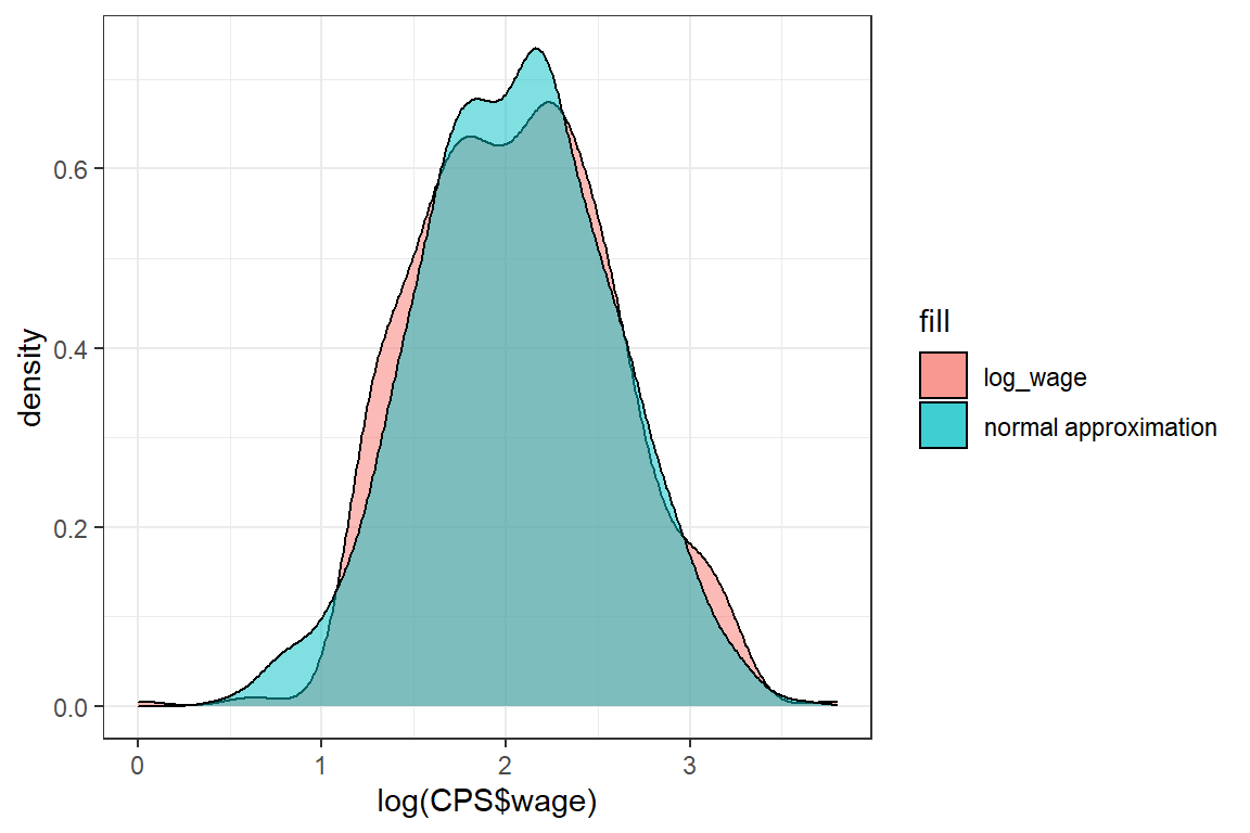

The approximation is better, but the normal distribution has fatter tails than the log(wage) distribution.