6 R implementation of the assignments 2019-2020

In this R tutorial you will implement the exercises from the assignment in R.

6.1 Assignment 1

The solution of the first assignment can be downloaded here.

6.1.1 Exercise 1

In the first exercise you computed a number of statistics for a distribution with cdf

\[ F_X(x) = \begin{cases} 0 & x < 0 \\ 1-0.5\cdot e^{-\beta\cdot x} & x \geq 0\end{cases}, \] for some \(\beta > 0\).

You can use the following function to simulate data from this distribution. Simulating from a given cdf will be covered in a later R tutorial.

simulate_assignment1 <- function(num_sim, beta) {
  rexp(num_sim, rate = beta) * (runif(num_sim) > 0.5)
}

# this code simulates 10 observations from this distribution with beta = 0.5
simulate_assignment1(10, beta = 0.5)

 [1] 4.31338 2.72700 0.00000 0.00000 0.00000 4.74313 0.00000 0.09661 0.23204
[10] 0.00000

Choose a value for \(\beta\) and simulate 10.000 observations from this distribution. Using this simulation:

Plot the empirical cdf of your simulation;
Compute \(P(X = 0)\);
Compute \(E(X)\);
Compute \(\sigma(X) = \sqrt{E((X - E(X))^2)}\).

Compare your answers with the solution of the assignment.

# set the seed for replicability when working with random numbers
set.seed(1) 
n <- 10000
beta = 0.1
simul <- simulate_assignment1(n, beta)

# @1
ggplot() +
  theme_bw() +
  stat_ecdf(aes(simul))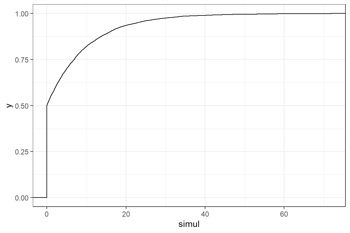

# @2
sum(simul == 0) / n

[1] 0.5018

#@3
mean(simul)

[1] 4.922

0.5/beta

[1] 5

#@4
sd(simul)

[1] 8.595

sqrt(0.75)/beta

[1] 8.66

Next, we calculate \(E((X-30)_+)\). To calculate an expected value of the form \(E(g(X))\) from a simulation, we compute

\[ \widehat{E(g(X))} = \frac{1}{n}\sum_{i=1}^n g(x_i),\] where \(x_i\) are our simulated outcomes from the random variable \(X\).

In the case of the mean \(E(X)\), \(g(x) = x\), i.e. the identity function. We implement this function in R as

identity <- function(x) {
  return(x)
}

mu = 1/n * sum(identity(simul))
print(mu)

[1] 4.922

You will now calculate the expected loss when there is a deductible of \(30\) using your simulated data.

Write a function deductible taking as input x (a vector containing the loss amounts) and d (the deductible) and returning a vector \(y\) with \(y_i = (x_i-d)_+ = \max(x_i-d, 0)\);
Test the function deductible that you defined in the previous step. What is the output for dedutible(c(500, 200), 300). Is your function working as expected? A common mistake in implementing the deductible function is a misunderstanding of the max function in R;

  # returns the maximum of 1, 3 and 2
  max(c(1, 3), 2)

[1] 3

  # returns a vector containing max(1, 2) and max(3, 2) 
  pmax(c(1, 3), 2)

[1] 2 3

Calculate \(E(X-30)_+\) for your simulated vector.

deductible <- function(x, d)
{
  return(pmax(x-d, 0))
}

1/n * sum(deductible(simul, 30))

[1] 0.2519

0.5 * exp(-30*beta) / beta

[1] 0.2489

You will now calculate the remaining statistics from exercise 1.

\(E(X \wedge 30)\)
\(e_X(30)\)
\(VaR_{0.95}(X)\)

# @1
limit <- function(x, limit) {
  return(pmin(x, limit))
}

mean(limit(simul, 30))

[1] 4.67

0.5/beta * (1-exp(-30*beta))

[1] 4.751

# @2
simul_excess_30 <- simul[simul > 30] - 30
mean(simul_excess_30)

[1] 10.12

1/beta

[1] 10

# @3
quantile(simul, 0.95)

  95% 
22.91

-log(0.1)/beta

[1] 23.03

6.2 Assignment 2

6.2.1 Exercise 2

You will solve a slightly adapted version of this exercise. Assume that the number of claims, \(N\), for an insurance portfolio follows a Poisson distribution with mean \(\lambda= 10\). The sizes of these claims are independent and follow a Gamma distribution with mean 1000 and variance 90000.

In this exercise you will compute various statistics related to the total loss.

Create a single simulation for the aggregate loss \(S = X_1 + ... + X_N\).

set.seed(1)
lambda <- 10
mu <- 1000
sigmasq <- 90000;

# Simulate the number of claims from a Poisson distribution
N <- rpois(1, lambda)

We have to simulate N losses from a gamma distribution with mean 1000 and variance 90000. When we check the documentation of rgamma we see that the distribution is parametrized by a shape and scale parameter.

In the details section of the documentation, you find: \[shape = a, scale = s, E(X) = a*s \text{ and } Var(X) = a*s^2.\] From this you can compute: \[scale = \frac{Var(X)}{E(X)} \text{ and } shape = \frac{E(X)}{scale}\]

scale = sigmasq / mu
shape = mu / scale

# Simulate N losses from a gamma distribution
X <- rgamma(N, shape = shape, scale = scale)

S = sum(X)

You have now created a single simulation of \(S\). Using a for-loop, you can generate multiple simulations.

num_sim <- 1000

# create a vector for storing the result of the simulation
aggregated_loss <- rep(NA, num_sim) 

for(i in 1:num_sim) {
  # Add your code for a single simulation here
  N <- 
  X <- 
  S <- 
    
  aggregated_loss[i] <- S
}

You will now update the for-loop above to analyze the aggregated loss.

Complete the for-loop and generate 1000 simulations of the aggregated loss;
Use these simulations to compute the mean and standard deviation of the aggregated loss;
Assume that the insurer imposes an ordinary deductible of 750. Add the variables N_after_deductible and aggregated_loss_deductible in your simulation, which register the number of claims exceeding the deductible and the aggregate loss after imposing the deductible respectively;
Visualize the distribution of the number of claims before and after imposing the deductible;
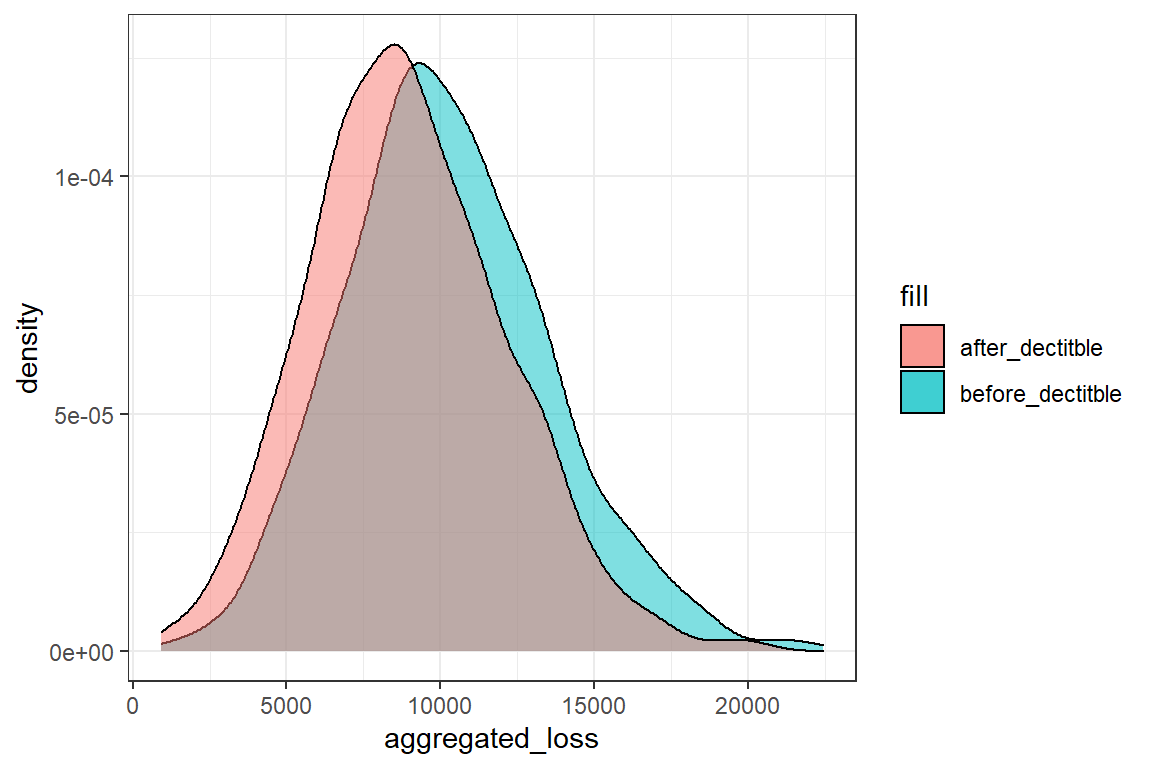
Compare the density of the aggregate loss before and after imposing the deductible.

# @1
num_sim <- 1000

# create a vector for storing the result of the simulation
aggregated_loss <- rep(NA, num_sim) 

for(i in 1:num_sim) {
  # Add your code for a single simulation here
  N <- rpois(1, lambda)
  X <- rgamma(N, shape = shape, scale = scale)
  S <- sum(X)
    
  aggregated_loss[i] <- S
}

# @2 
mean(aggregated_loss)

[1] 9999

sd(aggregated_loss)

[1] 3316

# @3
num_sim <- 1000

# create a vector for storing the result of the simulation
deductible <- 750
aggregated_loss <- rep(NA, num_sim) 
aggregated_loss_deductible <- rep(NA, num_sim) 
N <- rep(NA, num_sim)
N_after_deductible <- rep(NA, num_sim)

for(i in 1:num_sim) {
  # Add your code for a single simulation here
  N[i] <- rpois(1, lambda)
  X <- rgamma(N[i], shape = shape, scale = scale)
  S <- sum(X)
  
  aggregated_loss[i] <- S
  N_after_deductible[i] <- sum(X > deductible)
  aggregated_loss_deductible[i] <- sum(X[X > deductible])
}

df <- rbind(data.frame(count = N, method = 'before deductible'),
            data.frame(count = N_after_deductible, method = 'after_deductible'))

ggplot(df) +
  theme_bw() +
  geom_bar(aes(count, fill = method, y = ..prop.., group = method), position = position_dodge())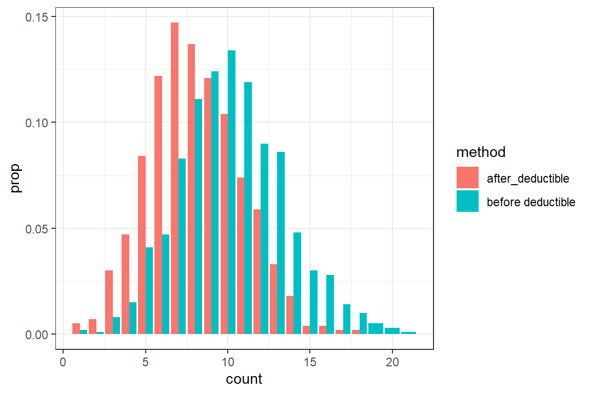

ggplot() +
  theme_bw() +
  geom_density(aes(aggregated_loss, fill = "before_dectitble"), alpha = .5) + 
  geom_density(aes(aggregated_loss_deductible, fill = "after_dectitble"), alpha = .5)